Principle components analysis (PCA) with `scikit-learn`¶

scikits-learn is a premier machine learning library for python, with a very easy to use API and great documentation.

In [1]: import mdtraj as md

In [2]: from sklearn.decomposition import PCA

Lets load up our trajectory. This is the trajectory that we generated in the “Running a simulation in OpenMM and analyzing the results with mdtraj” example.

In [3]: traj = md.load('ala2.h5')

In [4]: print traj
<mdtraj.Trajectory with 100 frames, 22 atoms>

Create a two component PCA model, and project our data down into this reduced dimensional space. Using just the cartesian coordinates as input to PCA, it’s important to start with some kind of alignment.

In [5]: pca1 = PCA(n_components=2)

In [6]: traj.superpose(traj, 0)
Out[6]: <mdtraj.Trajectory with 100 frames, 22 atoms at 0x10551bdd0>

In [7]: reduced_cartesian = pca1.fit_transform(traj.xyz.reshape(traj.n_frames, traj.n_atoms * 3))

In [8]: print reduced_cartesian.shape
(100, 2)

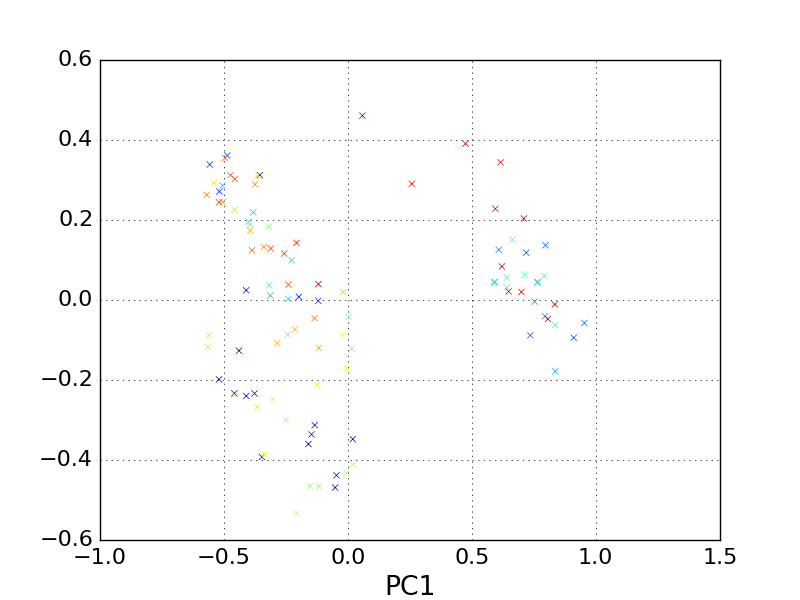
Now we can plot the data on this projection.

In [9]: import matplotlib.pyplot as pp

In [10]: pp.figure()
Out[10]: <matplotlib.figure.Figure at 0x10f589cd0>

In [11]: pp.scatter(reduced_cartesian[:, 0], reduced_cartesian[:,1], marker='x', c=traj.time)
Out[11]: <matplotlib.collections.PathCollection at 0x10e88a050>

In [12]: pp.xlabel('PC1')
Out[12]: <matplotlib.text.Text at 0x10f5a3c10>

In [13]: pp.ylabel('PC2')
Out[13]: <matplotlib.text.Text at 0x10e856d90>

In [14]: pp.title('Cartesian coordinate PCA: alanine dipeptide')
Out[14]: <matplotlib.text.Text at 0x10e90c610>

In [15]: cbar = pp.colorbar()

In [16]: cbar.set_label('Time [ps]')

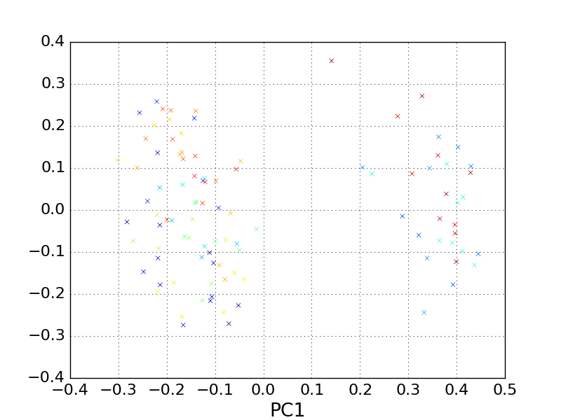
Lets try cross-checking our result by using a different feature space that isn’t sensitive to alignment, and instead to “featurize” our trajectory by computing the pairwise distance between every atom in each frame, and using that as our high dimensional input space for PCA.

In [17]: pca2 = PCA(n_components=2)

In [18]: from itertools import combinations

this python function gives you all unique pairs of elements from a list

In [19]: atom_pairs = list(combinations(range(traj.n_atoms), 2))

In [20]: pairwise_distances = md.geometry.compute_distances(traj, atom_pairs)

In [21]: print pairwise_distances.shape
(100, 231)

In [22]: reduced_distances = pca2.fit_transform(pairwise_distances)

In [23]: import matplotlib.pyplot as pp

In [24]: pp.figure()
Out[24]: <matplotlib.figure.Figure at 0x10d3d0750>

In [25]: pp.scatter(reduced_distances[:, 0], reduced_distances[:,1], marker='x', c=traj.time)
Out[25]: <matplotlib.collections.PathCollection at 0x10ed09690>

In [26]: pp.xlabel('PC1')
Out[26]: <matplotlib.text.Text at 0x10f598d10>

In [27]: pp.ylabel('PC2')
Out[27]: <matplotlib.text.Text at 0x10e87b110>

In [28]: pp.title('Pairwise distance PCA: alanine dipeptide')
Out[28]: <matplotlib.text.Text at 0x10f58a190>

In [29]: cbar = pp.colorbar()

In [30]: cbar.set_label('Time [ps]')

Principle components analysis (PCA) with scikit-learn¶

Principle components analysis (PCA) with `scikit-learn`¶